neuroGlia5D — Interactive 4D Label Editing Workflow

A0

Launch, Input Type Selection & Parameter Configuration

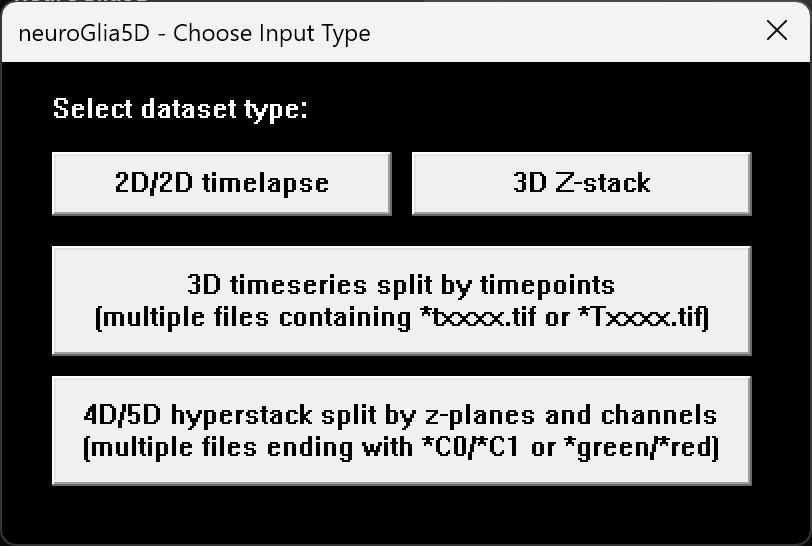
neuroGlia5D.exe prompts the user to choose a dataset type, then opens the parameter dialog (press S to save to parameters.json). All subsequent per-channel processing passes and output formats are controlled here.

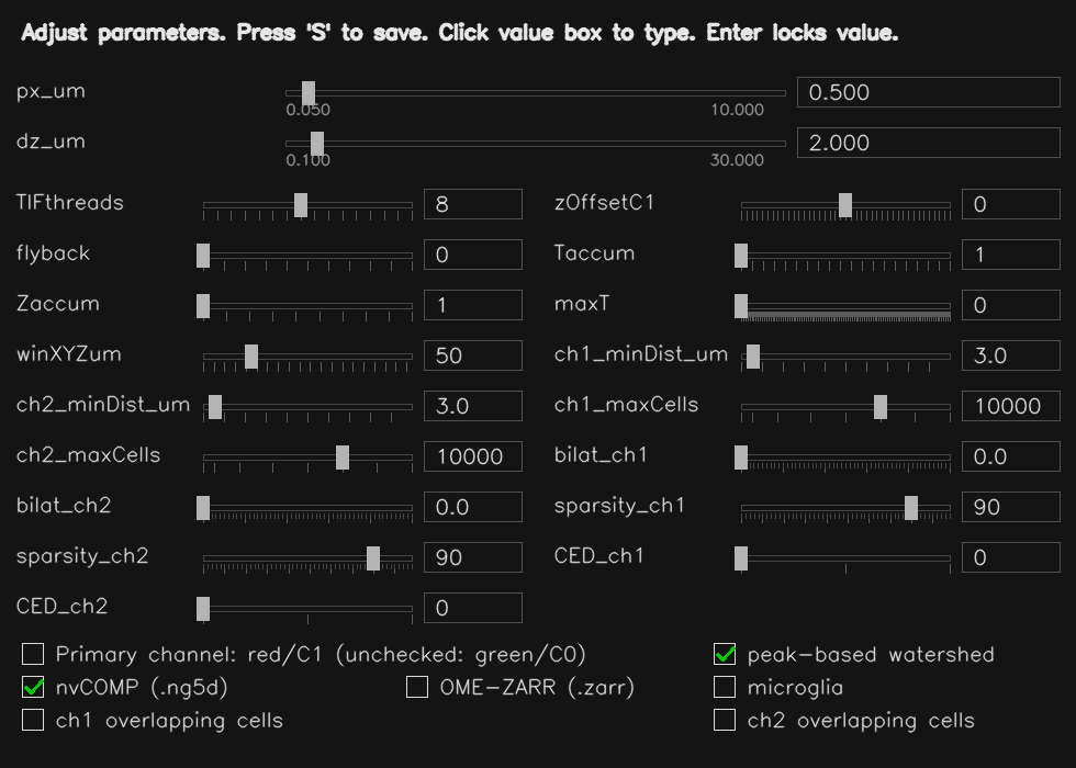
neuroGlia5D — Choose Input Type dialog — Input type selection dialog

neuroGlia5D Parameters dialog — Parameter configuration dialog (press S to save)

Key parameters:

px_um / dz_um — voxel size in XY and Z (µm); used to calibrate all object size and distance thresholds to physical units
ch1_minDist_um / ch1_maxSize_um — expected minimum and maximum object diameter in µm
sparsity_ch1 — controls how aggressively background is suppressed before segmentation (higher % = more aggressive removal)
bilat_ch1 — optional edge-preserving smoothing strength (0 = off); can sharpen object boundaries
CED_ch1 — structure enhancement filter strength (0 = off; 1 = gentle, 2 = normal, 3 = aggressive); useful for filamentous or branching morphologies
seed_merge_tol — controls how readily adjacent regions are merged into one object (higher = fewer, larger objects)
Taccum — number of raw timepoints to combine into each output frame
maxT — maximum intensity frames buffered before flushing to disk (0 = automatic)
winXYZum — spatial search radius (µm) used when filtering isolated or spurious labels
nvCOMP — enables GPU-compressed .ng5d streaming output

Tip — First-time setup

Start by setting px_um and dz_um to your microscope's calibrated voxel size. Set ch1_minDist_um to roughly the expected cell or nucleus diameter in µm. Leave all other parameters at their defaults for the first run, then review the output label statistics and the rejected-signal file saved at the first timepoint to decide if any adjustments are needed.

A1

Step 1 — Parallel Multi-Threaded TIFF / Stack Loading

For each output timepoint, neuroGlia5D loads the corresponding raw z-stacks in parallel across multiple CPU threads and transfers them to the GPU. Loading is parallelised across Z-planes or timepoint files depending on the input dataset type, minimising total I/O time regardless of stack size.

3D timeseries per file: threads work across timepoints simultaneously.
4D/5D hyperstacks: threads work across Z-planes of the same stack simultaneously.
Zaccum > 1: consecutive source z-planes are combined into a single output plane on the GPU (useful for anisotropic datasets).
Intensity clipping and threshold normalisation are applied on the GPU immediately after loading.
Insufficient VRAM is detected early; the pipeline aborts with a clear error message before processing begins.

A2

Step 2 — XY Bounding-Box Crop + Adaptive Background Subtraction

neuroGlia5D automatically determines the tightest XY bounding box enclosing the fluorescent signal, using the first timepoint as a reference. This crop region is then applied to all subsequent timepoints, eliminating empty border voxels and reducing memory and compute requirements.

Multiple automatic threshold methods are combined adaptively for robust detection across diverse sample types.
Small isolated bright artefacts are excluded from the bounding box calculation.

Adaptive background subtraction:

Background is progressively removed using a multi-scale blockwise approach. The process iterates until foreground sparsity reaches the target set by sparsity_ch1. A stall-detection mechanism automatically escalates aggressiveness if progress slows, and stops safely before over-subtracting genuine signal.

A3

Step 3 — Volume Pre-processing: Noise Removal, Structure Enhancement & Smoothing

The loaded frames are combined into a single 3D volume per timepoint. Isolated noise voxels are then removed using 3D connectivity analysis before segmentation.

Optional structure enhancement (CED_ch1 > 0):

Enhances filament and vessel continuity, producing cleaner segmentation boundaries for branching or tubular structures. Three strength levels are available: 1 = gentle, 2 = normal, 3 = aggressive.

Optional edge-preserving smoothing (bilat_ch1 > 0):

Applied per Z-plane to reduce noise while preserving object boundaries. If smoothing produces new isolated fragments, they are automatically cleaned up. If the result is unexpectedly sparse, the pipeline retries with a conservative smoothing strength automatically.

A4

Step 4 — Automatic Algorithm Selection + 3D Watershed Segmentation

At the first timepoint, neuroGlia5D runs an automatic calibration pass to select the segmentation algorithm best matched to the dataset's cell morphology. The choice is locked in for the rest of the timeseries, ensuring consistent segmentation across all timepoints.

Microglia mode: algorithm tuned for sparse branching morphology.
Overlapping mode: algorithm tuned for densely packed or contacting cells.
Default (auto): both candidate algorithms are evaluated on the first timepoint; the one whose average detected object size best matches the expected cell size (ch1_minDist_um) is selected automatically.

The primary algorithm fills the large majority of foreground. A secondary pass automatically fills any remaining unlabeled regions. A final cleanup loop recovers remaining bright blobs within the expected size range.

A5

Step 5 — Label Statistics, Nearest-Neighbour Distances & Isolation Filter

After segmentation, per-label statistics are computed on the GPU and used to intelligently discard noise, small fragments, and spatially isolated outliers.

Per-label measurements include: volume, mean and peak intensity, shape descriptors, and bounding box.
Nearest-neighbour distances between adjacent labels are computed in physical units (µm) within the winXYZum search radius; a distance histogram is exported alongside the output for inspection.
Labels that are both smaller than expected and have no sufficiently large neighbours within winXYZum µm are automatically discarded as isolated noise.
Per-timepoint label statistics are saved as *_labelStats.csv alongside the output files.
At the first timepoint, discarded signal is saved separately so users can review what was filtered out.

A6

Step 6 — Asynchronous Streaming Output

Labels and intensity volumes are written to disk asynchronously in background threads, so processing of the next timepoint proceeds immediately without waiting for I/O to complete.

.ng5d: GPU-compressed output; the format is designed for fast streaming writes: each timepoint is compressed directly on the GPU and appended to the file without any full-file rewrite.
.ome.zarr: Compressed chunks appended per timepoint, compatible with standard Zarr viewers and the OME-NGFF ecosystem.
.tif: Multi-page LZW TIFF, readable by ImageJ/FIJI and other standard tools.
All three formats can be written simultaneously when the corresponding checkboxes are enabled.
Intensity frames are buffered for up to maxT timepoints before being flushed, keeping peak memory usage bounded.

.ng5d: designed for GPU-accelerated workflows

OME-ZARR is an excellent open standard for data exchange and interoperability. The .ng5d format is neuroGlia5D's native format, optimised for interactive GPU-accelerated editing of large 4D volumes. Key advantages over generic formats:

Compressed data is kept in host RAM; decompression happens directly on the GPU on demand; only the active tile's uncompressed data ever occupies VRAM at one time.
Any dataset size opens regardless of GPU VRAM, since no data is decompressed up front — so even very large volumes are accessible immediately.
Each timepoint is appended independently, so both streaming output (during segmentation) and incremental saving (during editing) are O(1) per timepoint with no full-file rewrite.
Automatic codec selection at write time: the best available GPU compression is chosen based on the data characteristics, without user configuration.

OME-ZARR remains the recommended format for sharing data with external tools, pipelines, and collaborators.

1

Launch & File Selection

The user launches neuroGlia5Dviewer.exe. A file-open dialog appears; the user navigates to a directory containing 4D microscopy data and selects a file in any supported format: .tif .ng5d .ome.zarr

The file extension determines the reader: .tif → in-RAM TIFF reader, .ng5d → GPU-decoded directly to device memory, .ome.zarr → compressed chunk reader. Label files use *labels* in the name; intensity files use *fused*.

neuroGlia5Dviewer.exe │ ▼ File-open dialog │ ├─ user picks *labels.tif / .ng5d / .ome.zarr → go to Step 2 └─ user picks *fused.tif / .ng5d / .ome.zarr → go to Step 3 (both files expected)

2

Auto-Create Working Copy if Missing

When the user selects a labels file, the program checks whether a matching working copy (fused.*) already exists in the same directory, preserving the same format.

If the working copy does NOT exist: a copy of the labels file is created and renamed to the fused variant. This becomes the working copy that will be actively edited first purely in RAM, and then saved to disk after training and inference.
If the working copy already exists: no copy is made; both files are used as-is.

labels.* (selected — .tif, .ng5d, or .ome.zarr) │ ├─ fused.* exists? YES → use both │ └─ fused.* exists? NO │ ▼ copy labels.* → fused.* (new working copy, same format)

3

Multi-Format Loading & Role Assignment

Once both files exist, neuroGlia5D loads them into RAM using the format-appropriate reader:

.tif → decompressed in-RAM for instant Z/T navigation
.ng5d → GPU-decoded directly to device memory
.ome.zarr → Blosc-decompressed per chunk

Memory-mapped loading architecture — eliminating disk I/O during navigation

All three formats eliminate repeated disk reads during interactive Z/T navigation, each through a different mechanism rooted in the actual reader implementation:

.tif — Win32 memory-mapped file → resident RAM buffer

For stacks larger than 64 MB, the TIF loader uses the Windows memory-mapped file API, letting the kernel stream the file into a single contiguous host buffer in one sequential pass. Smaller files use a buffered per-thread read. Either way, once the load completes, the TIFF decoder is bound to the in-RAM buffer via custom I/O hooks. Every subsequent Z-plane or timepoint seek operates entirely in RAM. No disk activity occurs during navigation.

.ome.zarr — chunk-resident host buffer

The OME-ZARR reader loads all chunk files on initial load. Each chunk is Blosc-decompressed on the CPU and assembled into a contiguous host buffer. After this single loading pass, the full dataset lives in RAM and Z/T navigation requires no further disk access. The Blosc decompression happens once at load time, not on every slice access.

.ng5d — VRAM-resident compressed blobs → zero CPU decompression

The .ng5d engine reads compressed timepoint blobs sequentially from disk once, transferring each blob host-to-device into VRAM. During navigation, a GPU decompression kernel decompresses directly on-GPU into the output buffer. No CPU is involved, no PCIe transfer is needed per access, and no disk is touched after the initial load.

How this compares to other tools

Property	ImageJ / Fiji Virtual Stack	napari / dask Dask array	neuroGlia5D .tif / .zarr / .ng5d
Data after open	Nothing cached — disk on every slice	Lazy graph — disk on first access per chunk	Full dataset in RAM or VRAM after one load pass
Disk I/O during navigation	Every slice seek triggers a read	Re-reads on cache miss; cache is bounded	Zero — all navigation is RAM or VRAM resident
Decompression thread	CPU (or none for uncompressed TIF)	CPU — dask worker thread pool	.ng5d: GPU kernel only — CPU uninvolved
GPU path for intensity data	None — CPU / Java heap only	Optional via cupy; not default	Native — .ng5d decompresses straight to device buffer
Large file strategy	Virtual paging — always disk-backed	Chunked lazy load — CPU decompresses on demand	Win32 memory-mapped file API (TIF) or VRAM blobs (.ng5d)
4D timeseries navigation latency	Disk-limited — ms per slice on HDD	Dask scheduler overhead + disk on miss	RAM or VRAM speed — sub-ms per timepoint

ImageJ Virtual Stack and napari Dask are designed for exploratory analysis on arbitrarily large data that may exceed RAM. neuroGlia5D trades that generality for interactive speed: the full working dataset is loaded once up front, making repeated navigation, GPU rendering, and brush-stroke editing operate at memory bandwidth rather than disk bandwidth.

Regardless of input format, data is assigned to two roles:

labels.* → original / read-only reference. Kept in RAM solely for restore operations (undo to original state). Never written to.
fused.* → active working copy. This is the data that is viewed, edited, and eventually saved back to disk.

labels.* ── auto-detect format ──▶ read-only reference (for restore) ╲ ╲ both loaded into RAM ╲ fused.* ── auto-detect format ──▶ active working copy (view, edit, save) │ ▼ Interactive viewer

The viewer handles all GPU-based viewing and editing, but first, the 4D region-of-interest must be tiled to fit into VRAM (Step 4).

4

Adaptive 4D Tiling to Fit VRAM

Before loading the viewer, neuroGlia5D determines the tightest bounding ROI that encloses all labelled voxels across every z-plane and every timepoint, computed from the per-label bounding boxes saved during segmentation:

Global min/max of x, y, z across all labels and all timepoints → cropped ROI dimensions (W × H × D × T).

Each voxel must be stored twice on the GPU: once as uint16 intensity and once as uint32 label, totalling 6 bytes/voxel. The tiling logic proceeds as follows:

Advantage of .ng5d over .tif and .ome.zarr when working with large datasets

When a .ng5d file is loaded, the compressed data is kept in host RAM and decompressed directly on the GPU on demand, so only the active tile ever occupies uncompressed VRAM at any one time. Because the compressed representation is much smaller than the raw voxels, a single GPU can hold far more of the dataset in VRAM simultaneously compared to loading from .tif or .ome.zarr, where data must be fully decompressed before being transferred to the GPU.

GPU-native decompression is also significantly faster than the CPU-based codecs used for TIFF (LZW) and Zarr (Blosc-LZ4). The GPU processes all chunks of a tile in parallel, whereas CPU decompression is serial or limited to a small thread pool, so tile-switch latency noticeably shorter when working interactively on large 4D volumes.

Tile properties:

All tiles have the same total voxel count (uniform partitioning).
Adjacent tiles share an overlap region so that labels straddling tile boundaries are fully visible from either tile.
The tile grid is selected automatically based on the dataset aspect ratio and available VRAM. Supported layouts range from 1×1 up to 4×4 (16 tiles).
If spatial tiling alone cannot fit all timepoints, the viewer switches to adaptive time-windowing: a sliding window of timepoints is kept resident in VRAM and swapped seamlessly as the user scrolls. The user never sees an error message.

15 % overlap between adjacent tiles:

Tile A

15 %

Tile B

Example tile layouts (active tile shown in white):

1 × 1

1

2 × 1

1

2

1 × 2

1

2

2 × 2

1

2

3

4

3 × 2

1

2

3

4

5

6

3 × 3

1

2

3

4

5

6

7

8

9

4 × 2

1

2

3

4

5

6

7

8

4 × 3

1

2

3

4

5

6

7

8

9

10

11

12

3 × 4

1

2

3

4

5

6

7

8

9

10

11

12

4 × 4

1

2

3

4

5

6

7

8

9

10

11

12

13

14

15

16

Data Buffering panel (visible in the viewer sidebar)

The sidebar always shows the current memory state so you know exactly how much data is buffered and how much remains:

Data Buffering: VRAM loaded: X MB (active tile, resident timepoints — uncompressed on GPU) RAM loaded: Y MB (full dataset compressed in host RAM) VRAM+RAM loaded: Z MB (total memory in use) Pending to VRAM: W MB (non-resident timepoints or non-active tiles) Pending disk→RAM: 0 B (all source data is already in RAM)

VRAM loaded: uncompressed intensity + label data for the active tile currently on the GPU
RAM loaded: the full compressed working dataset resident in host RAM
Pending to VRAM: data not yet on the GPU (other spatial tiles, or timepoints outside the current window in adaptive mode)
Pending disk→RAM: always 0; all source data is loaded into host RAM at startup

5

Tile Navigation via Checkerbox Window

A small, always-on-top checkerbox window is displayed at the top-right corner of the screen. It mirrors the tile grid layout. The active tile is drawn as a white box; inactive tiles are dark.

Click an inactive tile → the viewer closes, the selected tile's data is decompressed from host RAM and uploaded to the GPU, then the viewer reopens with the new tile.
All unsaved edits to the previous tile are flushed back to the compressed host buffer before switching.

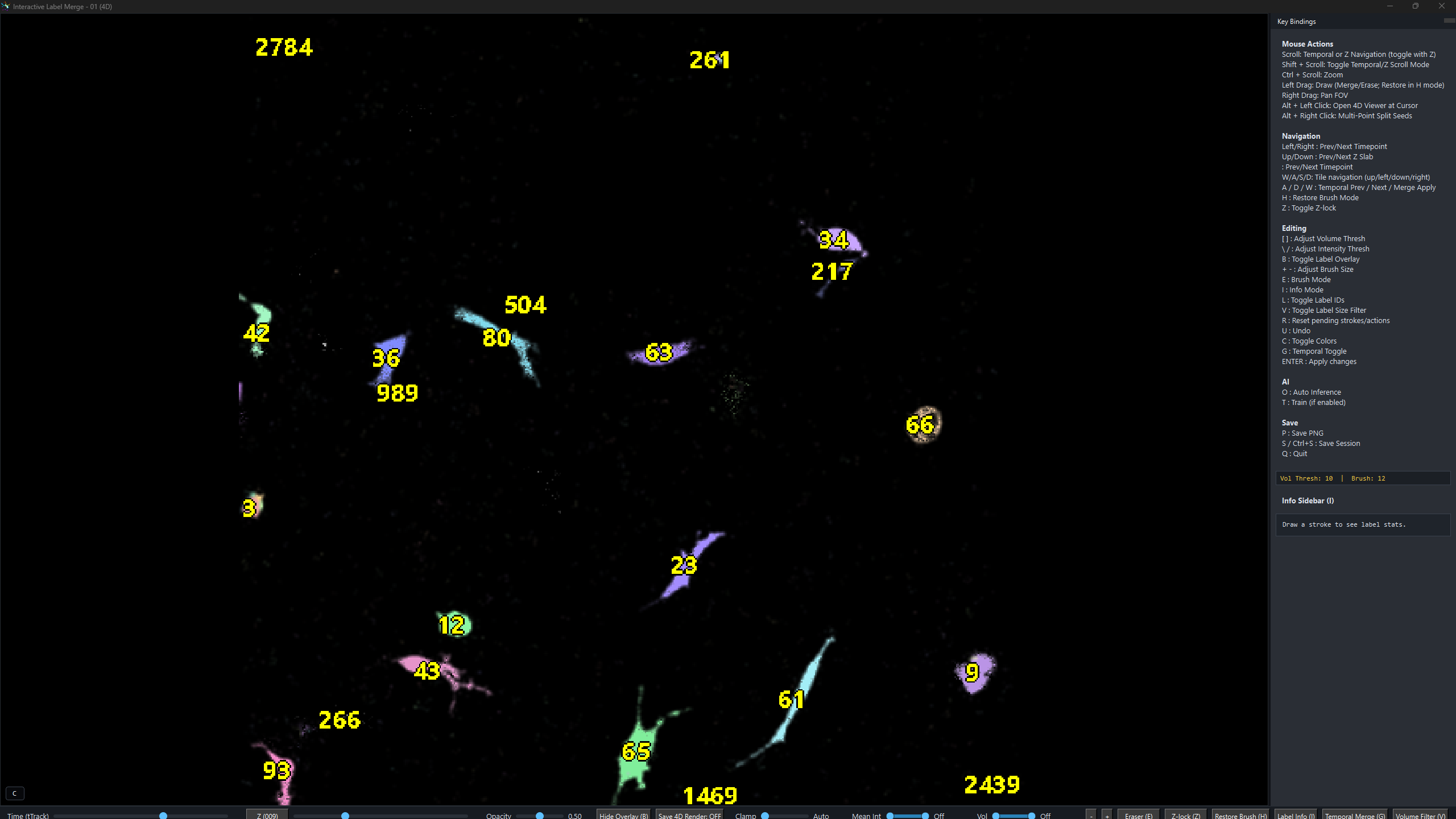
┌────────────────────────────────────────────────────────────┐ │ Main viewer (active tile) │ │ │ │ 4D volume + labels from active tile rendered on GPU │ │ ┌──────┐ │ │ │■ □ □ │ │ ← checkerbox │ │□ □ □ │ │ (top-right) │ │□ □ □ │ │ │ └──────┘ │ └────────────────────────────────────────────────────────────┘ User clicks another tile box: │ ▼ 1. Flush current tile edits → compressed host buffer 2. Decompress new tile ROI → host buffers 3. Upload to GPU (intensity + labels) 4. Reopen viewer with new tile

6

Interactive Label Editing Operations

Inside the viewer, the user can seamlessly scroll through z-planes and timepoints. The user draws brush strokes of three colours with adjustable widths:

White brush (left-drag) — marks labels for 3D merge

Red brush (left-drag with E toggle) — marks labels for erase (set to 0)

With V active: only erases labels smaller than the current volume threshold — useful for removing small debris without touching large cells

Blue brush (left-drag with H toggle) — restore only: reverts selected labels to their original watershed state

Z Z-lock — toggles a modified behaviour for all three brushes:

Erase: restricted to the current Z-slice only — does not erase the label through the full 3D volume
Merge: instead of merging the painted labels directly, the viewer searches the z-planes immediately below the current slice for the best matching adjacent label and merges those — designed for stitching labels that are adjacent across a Z-boundary but do not overlap
Split: same algorithm, but recorded as a Z-constrained split in the annotations file

While painting with the white brush, the right-hand stats panel updates live for every label touched by the stroke, helping you decide what is under the brush and what should or should not be merged. Only adjacent label pairs are recorded (not all-to-all cliques), preventing false-positive merges.

Mouse controls:

Left drag — paint white / red / blue brush stroke (mode depends on E / H toggle)
Right drag — pan the field of view (when canvas is larger than window)
ALT + Left click — launch 4D RGB render: crops a bounding box around the clicked label (+ 30 µm XY and Z padding), tracks the object across all timepoints, and opens an interactive volume render — tracked object shown in green, all other labels shown in red
ALT + Right click — multi-point split mode: click rough centroids of sub-cells inside one over-merged label (≥ 2 seeds required), then press Enter to apply an N-way Voronoi + intensity split — works even when original watershed boundaries are gone
Scroll — navigate timepoints
SHIFT + Scroll — temporarily switch to Z-slab navigation mode
CTRL + Scroll — zoom in / out, centered on mouse position

Keyboard:

E — toggle brush: WHITE (merge) / RED (erase)
H — toggle restore brush (BLUE; left-drag reverts labels to original)
G — toggle temporal merge mode (left-click links the same object across timepoints; each G press starts a new track)
Z — toggle Z-lock (fix the displayed Z-slab while scrolling timepoints)
V — toggle erase-size filter (erase only labels whose volume is below the threshold; also highlights small labels)
[ / ] — decrease / increase volume threshold for small-label highlighting and size-filtered erase
I / L — toggle label ID overlay (renders each label's numeric ID at its centroid)
O — auto-inference on all objects in the active tile; saves *_auto_annotations.json
B — toggle label overlay / raw intensity-only view
C — cycle label colours (random seed)
T — close viewer and launch PuzzleNet training from saved annotations (Step 7)
R — reset all pending strokes (does not apply anything)
U — undo last stroke (only available before pressing Enter)
P — export current view to PNG (*_interactive_Z000-ZZZ.png)
+ / − — increase / decrease brush stroke width
< / > — previous / next timepoint (instant when all timepoints are resident; seamlessly loads adjacent window if adaptive time-windowing is active)
W / A / S / D — tile navigation: move the active tile up / left / down / right in multi-tile mode
Enter — apply all pending operations (erase, merge, multi-point split, restore)
Ctrl+S — save to disk: flushes edited labels and labelStats to timestamped output files (never overwrites originals)
Q / ESC — quit (auto-saves annotations)

Bottom-left HUD: Every keyboard press and mouse click is echoed as a one-line status message (green text) in the bottom-left corner of the viewer, so the user always knows which action was last registered.

Automatic Label Stats Panel & Topology Analysis

As you paint with the white merge brush, the right-hand sidebar panel updates immediately for every label touched by the stroke. This helps the user see what is under the brush and decide which labels should or should not be merged. These per-label measurements are drawn from the *_labelStats.csv files and recomputed live after any edit:

┌───────────────────────────┬──────────────────────────────────────────────────┐ │ Measurement │ Description │ ├───────────────────────────┼──────────────────────────────────────────────────┤ │ Volume │ Voxel count for the label │ │ Position │ Bounding-box origin (x, y, z) │ │ Centroid │ Sub-voxel centre of mass (cx, cy, cz) │ │ Bounding box │ Tight axis-aligned box around the label │ │ Mean intensity │ Average raw fluorescence inside the label │ │ Peak intensity │ Brightest voxel inside the label │ │ Sum intensity │ Total signal across all voxels │ │ Intensity concentration │ Fraction of total signal in the brightest half │ │ PCA axis ratio │ Elongation: longest ÷ shortest principal axis │ │ Sphericity │ 1.0 = perfect sphere; lower = elongated / flat │ │ Fill factor │ Voxels ÷ bounding-box volume (compactness) │ │ Vesselness │ Tubularity score (useful for filamentous cells) │ │ Nearest-neighbour dist │ Surface distance to the closest other label (µm)│ │ Nearest-neighbour ID │ Label ID of the nearest neighbour │ └───────────────────────────┴──────────────────────────────────────────────────┘

In addition, neuroGlia5D computes topological structure metrics for the current merge-brush label set in real time and appends them at the bottom of the sidebar panel:

┌──────────────────────────────┬─────────────────────────────────────────────────┐ │ Topology Metric │ What it tells you │ ├──────────────────────────────┼─────────────────────────────────────────────────┤ │ β₀ (connected components) │ Number of distinct, separate objects │ │ β₁ (loops / holes) │ Number of enclosed cavities or tunnels in 3D │ │ Euler characteristic │ β₀ − β₁; single-number topological summary │ │ Skeleton edge count │ Number of branches in the 3D skeleton graph │ │ Mean skeleton degree │ Average connections per branch junction │ │ Rich-club coefficient │ Whether high-degree junctions cluster together │ │ Percolation threshold │ Distance (µm) at which objects form a cluster │ │ Fractal dimension │ Box-counting dimension of the label surface │ │ Sholl entropy │ Complexity of branching patterns with distance │ │ Orientation anisotropy │ Directional bias of the selected object group │ └──────────────────────────────┴─────────────────────────────────────────────────┘

These measurements are also saved alongside your output files:

*_labelStats.csv — per-label measurements for every object at each timepoint (produced during segmentation, Step A5)
*_topologyAdvanced_YYMMDDhhmmss.csv — full topology summary for a single timepoint (saved after each Ctrl+S)
*_topologyAdvanced4D_YYMMDDhhmmss.csv — time-series dynamics of topology metrics across all timepoints (Euler fluctuation, branch turnover, connectivity stability, and more)

These strokes and keys produce five distinct operations:

┌───────────────────┬───────────────────────────────────────────────┐ │ Operation │ Description │ ├───────────────────┼───────────────────────────────────────────────┤ │ ERASE │ Remove false-positive labels (set to 0) │ │ MERGE │ Fuse multiple labels into one (spatial, 3D) │ │ SPLIT │ N-way Voronoi+intensity split — ALT+RIGHT CLICK │ │ TEMPORAL_MERGE │ Link the same object's label across timepoints │ │ RESTORE │ Undo to original label from labels.tif │ └───────────────────┴───────────────────────────────────────────────┘

neuroGlia5D Interactive Label Merge viewer — Interactive Label Merge viewer with coloured segmentation labels overlaid on raw fluorescence data, with key-bindings sidebar and status bar.

4D RGB Render — ALT + Left Click on any label

Hold ALT and left-click any label to immediately launch the 4D RGB renderer for that object. neuroGlia5D crops a tight bounding box around the clicked label, adds user-specified padding in XY and Z, tracks the object across every timepoint, and opens a full GPU volume render with the tracked object in green and all other labels in red. The render below shows a single microglia imaged across multiple timepoints.

4D RGB render: tracked object (green) vs. surrounding labels (red). Rendered directly from GPU-resident label data without any export step.

Every operation is applied instantly on the GPU. Simultaneously, all information needed to replay/retrain that operation is appended to a JSON annotations file in the exact order the user applied them. Each entry records the operation type, timepoint, involved label IDs, seed coordinates (for splits), and a monotonic created_idx.

annotations.json (append-only, sequential) ───────────────────────────────────────────── [ { "type": "merge", "t": 3, "labels": [12, 45], "idx": 0 }, { "type": "erase", "t": 3, "labels": [7], "idx": 1 }, { "type": "split", "t": 5, "labels": [22, 99], "x": [110, 180], "y": [45, 90], "z": 12, "idx": 2 }, { "type": "temporal_merge", "timepoints": [3, 4, 5], "labels": [[12, 45], [12], [67, 89, 12]], ← sub-labels per timepoint "z_slices": [8, 8, 8], "idx": 3 }, { "type": "restore", "t": 3, "labels": [7], "idx": 4 }, ... ]

Sub-labels (temporal_merge): Each element in the labels array is itself an array listing the original constituent labels that were spatially merged (via the white brush) into the single fused label the user clicked when toggling G. For example, [[12, 45], [12], [67, 89, 12]] means: at t=3 the user clicked a label that was the result of merging original labels 12 and 45; at t=4 the label was unmerged (only 12); at t=5 the label was a fusion of 67, 89, and 12.

The user does not need to annotate every object in the 4D FOV. A representative subset is sufficient. The neural networks (Step 7) will generalise from these annotations.

7

Press `T` — Multi-Architecture AI Training

When the user presses T, neuroGlia5D reads all annotations collected so far and trains each specialised sub-network on its corresponding operation type. A minimum number of examples per category is required before training begins for that category; any category with too few annotations is deferred until more are collected. Operations are always trained in a fixed order so that artefact removal completes before spatial merge training begins, giving each network the cleanest possible training set.

① Adaptive Training Controller

Trained at the end of each session on the full sequence of user operations. Monitors accuracy and loss across training rounds and automatically adjusts the learning rate and training effort for each subsequent batch, making later sessions progressively more efficient.

② Split Network

Learns from your split annotations to predict where the 3D boundary between two touching objects should be drawn. When you place seed points on two distinct objects inside a fused label, this network determines the optimal dividing surface in 3D.

③ 4D Tracking Network

Learns from your temporal-merge annotations to recognise the same biological object across different timepoints. Produces consistent label identities throughout the timeseries, enabling accurate 4D cell tracking.

④ Artifact Detector

Learns from your erase annotations to recognise and suppress spurious segmentation labels. Trained once from the first set of erase examples in a session; the trained detector then automatically removes similar false positives across the rest of the dataset.

⑤ Spatial Merge Network

Learns from your merge annotations to predict which spatially adjacent label pairs represent the same biological object in 3D. Handles spatial fusion within a single timepoint; cross-timepoint linking is handled by the 4D Tracking Network.

User presses T │ ▼ Read annotations.json → group by operation type │ ├─ Too few examples in a category? → defer (collect more and press T again) │ ▼ Train each sub-network in order: ├─ Split annotations → update Split Network ├─ Erase annotations → update Artifact Detector (once per session) ├─ Merge annotations → update Spatial Merge Network └─ Temporal annotations → update 4D Tracking Network │ ▼ Run auto-inference on all label pairs in the current tile: ├─ Spatial: which adjacent labels should be merged? └─ Temporal: which labels across timepoints are the same object? │ ▼ Apply predicted merges → save tile │ ▼ Viewer reopens — AI predictions visible for user review │ End of session → Adaptive Controller trains on full operation sequence Weights saved to disk → reloaded automatically next session

After training completes, neuroGlia5D automatically runs inference on every label pair in the current tile: both spatial (merge candidates) and temporal (cross-timepoint identity). Predicted merges are applied to the label volume and the viewer reopens immediately so you can inspect the results. Continue annotating, correct any mistakes, switch tiles, and press T again to retrain. Learning is incremental: each session builds on the weights saved by the previous one.

Tip — How many annotations do you need?

You do not need to annotate every object. A representative sample is sufficient. Typically, 5–20 examples per operation type is enough to get started. The AI generalises from these to the rest of the dataset. Focus on the most visually obvious errors first, run training, inspect the results, then annotate further only where the AI still makes mistakes.

8

AI Architecture & GPU-Adaptive Scaling

neuroGlia5D’s neural network ensemble is purpose-built for large volumetric imaging data. Every component operates natively in 3D or 4D for full volumetric coverage. Unlike conventional pixel-centric pipelines, neuroGlia5D begins from segmented labels rather than raw voxel grids. This compact object-level representation, generated by the GPU segmentation engine, drastically reduces memory requirements while preserving structural fidelity. The networks are trained from scratch in real time on the GPU using a custom-built learning engine, without dependency on external ML frameworks such as PyTorch or TensorFlow, ensuring tight GPU integration, minimal overhead, and full architectural control.

Key highlights:

True 4D convolutions: the convolutional backbone processes raw (X, Y, Z, T) patches as native 4D tensors with 4D kernels, capturing spatio-temporal features that 2D or even 3D networks cannot represent.
Multi-head self-attention: after convolution, label embeddings pass through multiple layers of multi-head self-attention, allowing the network to model complex inter-label relationships before making merge/split decisions.
Fusion head with pairwise features: element-wise products and absolute differences of embeddings are combined with scalar geometric features (centroid distance, volume ratio, temporal separation) and passed through a multi-layer fusion network to produce a single merge probability.
Full GPU residency: the entire inference pipeline (ROI extraction → 4D convolution → attention → fusion → prediction) runs end-to-end on the GPU without any host round-trips, using 32 custom CUDA kernels.
Per-operation specialisation: each user operation type (merge, split, erase, temporal link, restore) is routed to its own specialised network, avoiding the compromises of a single monolithic model.

VRAM-adaptive scaling:

Both the interactive viewer and the AI inference pipeline automatically adapt to the amount of GPU VRAM available on the user's hardware:

Viewer tiling: the volume is partitioned into as few tiles as possible given the available VRAM (see Step 4). Layouts range from 1×1 up to 4×4. A GPU with more VRAM can often display the entire volume in a single tile, eliminating boundary artefacts entirely. With the adaptive time-window fallback, every dataset opens regardless of GPU size.
AI field-of-view: the spatial extent of the region extracted around each label pair scales proportionally to available VRAM: more VRAM gives the networks more surrounding context, improving decision accuracy. The temporal window also expands when memory permits.

The minimum VRAM requirement is 8 GB. Users with 16 GB, 24 GB, or 32 GB GPUs benefit substantially: the AI sees a dramatically larger neighbourhood around every label, and the viewer can fit more (or all) of the volume into a single tile. This scaling happens automatically at startup with no user configuration required. For improved accuracy, it is recommended that instead of using the same network weights for drastically different datasets, the user should train separate networks for each sample-type. For instance, network weights obtained from sparse microglial datasets can work well for sparse neuronal datasets, but not for dense crowded environments, where it needs to be more conservative on fusion and artifact detection, and would typically require more training labels to achieve comparable accuracy as less crowded cellular environments. For such special cases, the user can maintain multiple sets of weights on disk and load the appropriate ones before training/inference. The same network weights should work well for datasets with slightly different resolution and signal-to-noise ratio, but a network trained on a 24 GB GPU will not perform well if loaded onto an 8 GB GPU due to significantly smaller field-of-view, but will perform decently on a 16 GB GPU.

Viewer (tiling) budget = available VRAM tile count: 1×1 → 2×1 → 2×2 → … → 4×4 → adaptive time-window ↑ fewer tiles = larger FOV per tile = better user experience AI (ROI limits) available VRAM is shared between viewer and AI networks larger VRAM → larger inference context → more accurate predictions GPU VRAM Viewer tiles AI context Experience ────────── ──────────── ───────────── ────────── 8 GB 2×2 – 4×4 small baseline 12 GB 1×2 – 2×2 medium good 16 GB 1×1 – 2×1 large very good 24 GB 1×1 larger excellent 32 GB+ 1×1 maximum maximum

9

Multi-Format Output Pipeline

When saving (Ctrl+S), neuroGlia5D v1.4 writes the edited volume in up to three formats based on user preferences set via the GUI checkboxes. The format priority ensures the fastest-to-reload option is preferred.

Edited volume
GPU → host

➜

.ng5d
if enabled ✔

➜

.ome.zarr
if ZARR ✔

➜

.tif
always

.ng5d: GPU-compressed format; codec is selected automatically based on data characteristics. Fastest reload for subsequent sessions.
.ome.zarr: Zarr v2 directory store, compressed. Incremental per-timepoint chunks. Interoperable with napari, FIJI, BigDataViewer.
.tif: LZW-compressed MemTIFF. Universal fallback, compatible with all bioimage tools.

Ctrl+S pressed │ ├─ .ng5d checkbox? YES → write .ng5d (GPU-compressed, automatic codec selection) │ ├─ ZARR checkbox? YES → write .ome.zarr per timepoint │ └─ always → write .tif (LZW fallback)

∞

End-to-End Summary

neuroGlia5Dviewer.exe │ ▼ select labels.* or fused.* (.tif / .ng5d / .ome.zarr) │ ├─ ensure both files exist (copy if needed) │ ▼ Load files into host RAM: │ ├─ load labels.* → read-only reference (for restore operations) ├─ load fused.* → active working copy (view, edit, save) │ ├─ compute global ROI from label bounding boxes across all T ├─ determine tile layout to fit VRAM (1×1 … 4×4; adaptive time-window if needed) │ ▼ ┌──────────────────────────────────────────────┐ │ Interactive viewer (active tile) │ ◄── tile loop │ │ │ Intensity + label volumes on GPU │ │ Navigate z / t, draw brush strokes │ │ Operations: erase, merge, split, │ │ temporal_merge, restore │ │ All ops → annotations.json (sequential) │ │ │ │ Press T → train all networks → auto-infer │ │ → apply merges → reopen viewer │ │ Press O → auto-inference on all objects │ │ Merge brush → auto stats for labels under brush │ │ Press G → temporal merge (4D linking) │ │ Ctrl+S → save to disk (multi-format) │ │ Click checkerbox → switch tile │ │ Bottom-left HUD shows last action │ └──────────────────────────────────────────────┘ │ ▼ Save → .ng5d (GPU-compressed) │ .ome.zarr (compressed) │ .tif (LZW)

neuroGlia5D v1.4 Workflow

Segmentation Pipeline

Launch, Input Type Selection & Parameter Configuration

Step 1 — Parallel Multi-Threaded TIFF / Stack Loading

Step 2 — XY Bounding-Box Crop + Adaptive Background Subtraction

Step 3 — Volume Pre-processing: Noise Removal, Structure Enhancement & Smoothing

Step 4 — Automatic Algorithm Selection + 3D Watershed Segmentation

Step 5 — Label Statistics, Nearest-Neighbour Distances & Isolation Filter

Step 6 — Asynchronous Streaming Output

Interactive Viewer & AI Training (neuroGlia5Dviewer.exe)

Launch & File Selection

Auto-Create Working Copy if Missing

Multi-Format Loading & Role Assignment

Adaptive 4D Tiling to Fit VRAM

Tile Navigation via Checkerbox Window

Interactive Label Editing Operations

Automatic Label Stats Panel & Topology Analysis

Press `T` — Multi-Architecture AI Training

① Adaptive Training Controller

② Split Network

③ 4D Tracking Network

④ Artifact Detector

⑤ Spatial Merge Network

AI Architecture & GPU-Adaptive Scaling

Multi-Format Output Pipeline

End-to-End Summary

neuroGlia5D v1.4 Workflow

Segmentation Pipeline

Launch, Input Type Selection & Parameter Configuration

Step 1 — Parallel Multi-Threaded TIFF / Stack Loading

Step 2 — XY Bounding-Box Crop + Adaptive Background Subtraction

Step 3 — Volume Pre-processing: Noise Removal, Structure Enhancement & Smoothing

Step 4 — Automatic Algorithm Selection + 3D Watershed Segmentation

Step 5 — Label Statistics, Nearest-Neighbour Distances & Isolation Filter

Step 6 — Asynchronous Streaming Output

Interactive Viewer & AI Training (neuroGlia5Dviewer.exe)

Launch & File Selection

Auto-Create Working Copy if Missing

Multi-Format Loading & Role Assignment

Adaptive 4D Tiling to Fit VRAM

Tile Navigation via Checkerbox Window

Interactive Label Editing Operations

Automatic Label Stats Panel & Topology Analysis

Press T — Multi-Architecture AI Training

① Adaptive Training Controller

② Split Network

③ 4D Tracking Network

④ Artifact Detector

⑤ Spatial Merge Network

AI Architecture & GPU-Adaptive Scaling

Multi-Format Output Pipeline

End-to-End Summary

Press `T` — Multi-Architecture AI Training